19 Expression heatmaps
One of the major ways to assess cell identities in your data is to query the expression of several marker genes across the different clusters in you data. While computing FeaturePlots might be a very good idea to assess this, sometimes one wants to query multiple features at the same time. This can be achieved with SCpubr::do_ExpressionHeatmap().
This kind of heatmaps can be easily computed using SCpubr::do_EnrichmentHeatmap():
19.1 Single grouping variable
# Define list of genes.
genes <- c("IL7R",
           "CCR7",
           "CD14",
           "LYZ",
           "S100A4",
           "MS4A1",
           "CD8A",
           "FCGR3A",
           "MS4A7",
           "GNLY",
           "NKG7",
           "FCER1A",
           "CST3",
           "PPBP")

# Default parameters.
p <- SCpubr::do_ExpressionHeatmap(sample = sample,
                                  features = genes,
                                  viridis_direction = -1)
p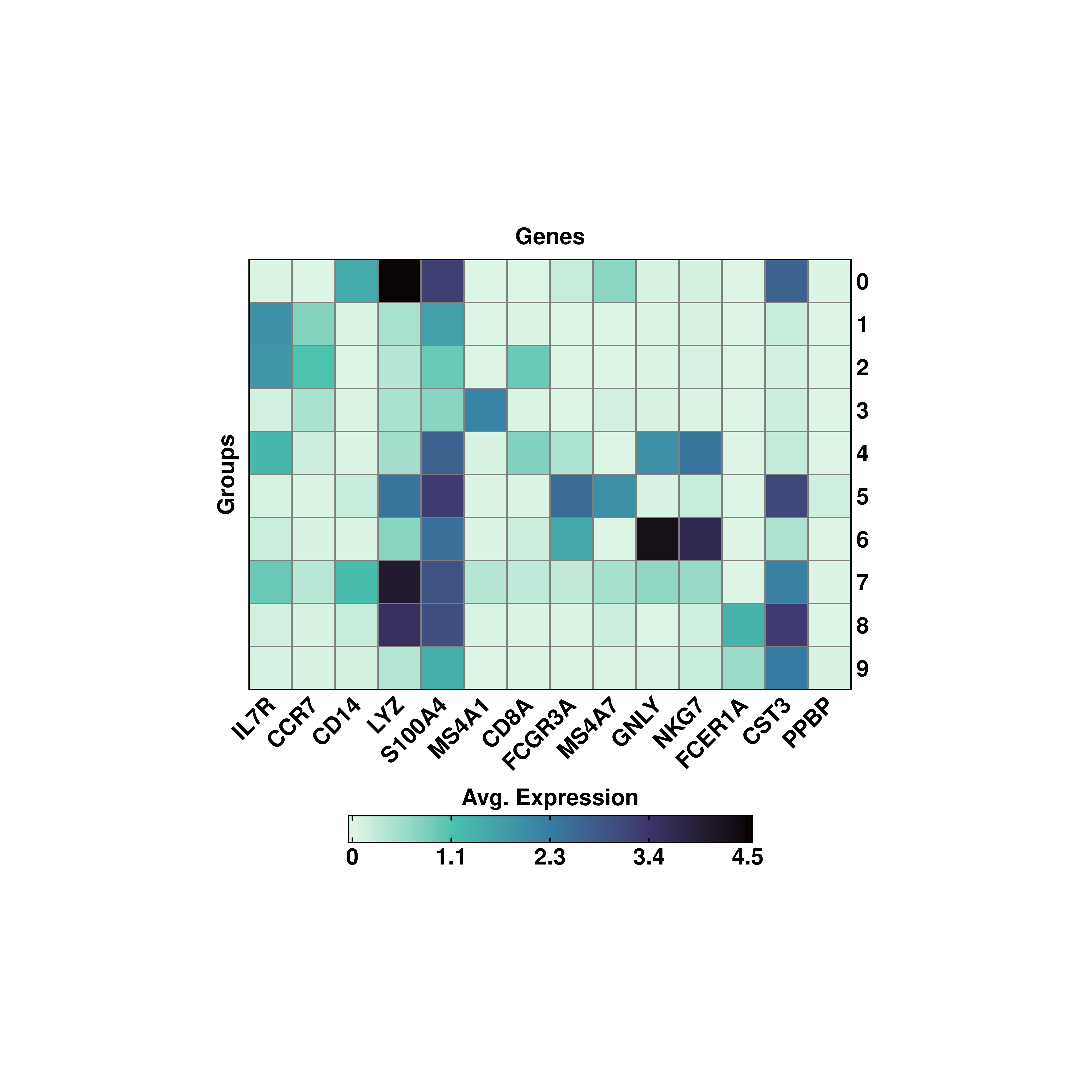
In these cases, inverting the color scale with viridis_direction = -1 is the best choice as makes it easir to identify dark colors in the heatmap and they stand out more than it would do when it comes to using light colors on dark background.
By default, SCpubr::do_ExpressionHeatmap aggregates the values by the current identity. However, other metadata variables can be used to aggregate for. For this, provide the name to group.by parameter.
# Custom aggregated values.
p <- SCpubr::do_ExpressionHeatmap(sample = sample,
                                  features = genes,
                                  group.by = "annotation",
                                  viridis_direction = -1)
p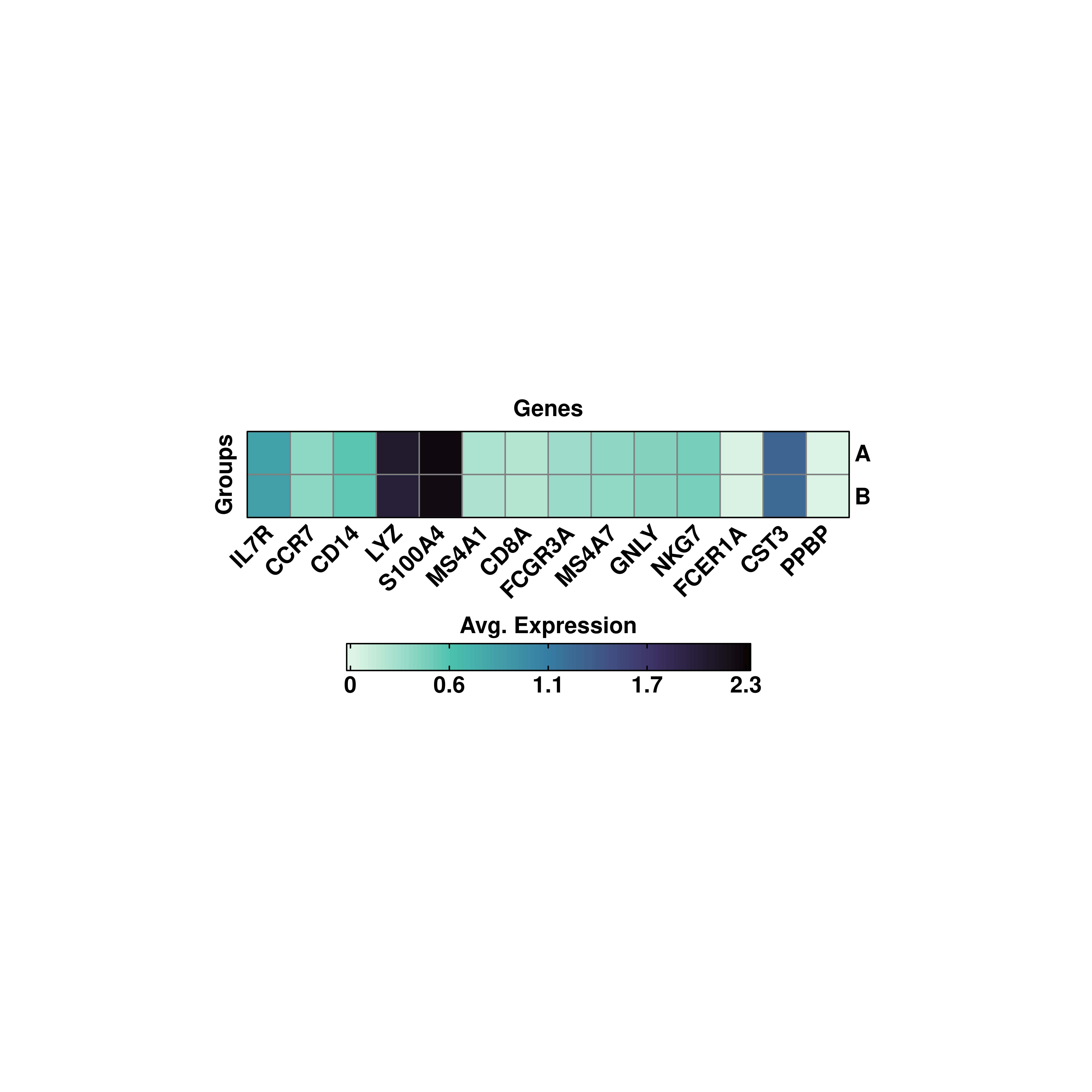
19.2 Several groupoing variables
However, more than one variable can be passsed at the same time to group.by:
# Group by several variables.
p <- SCpubr::do_ExpressionHeatmap(sample = sample,
                                  features = genes,
                                  group.by = c("seurat_clusters", "orig.ident", "annotation"),
                                  viridis_direction = -1)
p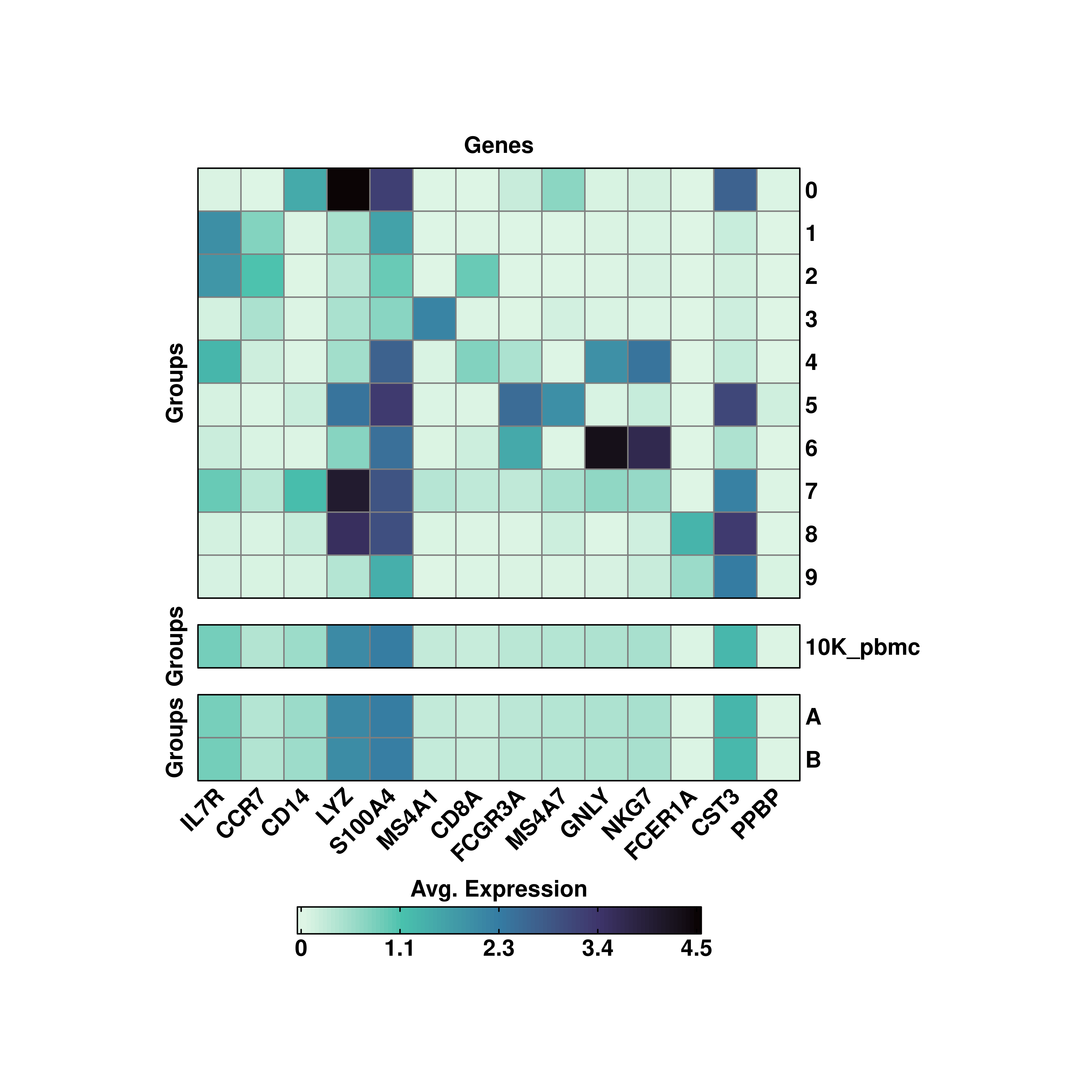
One can also customize the group titles by providing as many characters as variables in group.by to row_title:
# Custom aggregated values.
p <- SCpubr::do_ExpressionHeatmap(sample = sample,
                                  features = genes,
                                  group.by = c("seurat_clusters", "orig.ident", "annotation"),
                                  row_title = c("A", "B", "C"),
                                  viridis_direction = -1)
p
19.3 Transpose the heatmaps
The heatmaps can be transposed using flip = TRUE.
# Transposing the matrix.
p <- SCpubr::do_ExpressionHeatmap(sample = sample,
                                  features = genes,
                                  flip = TRUE,
                                  viridis_direction = -1)
p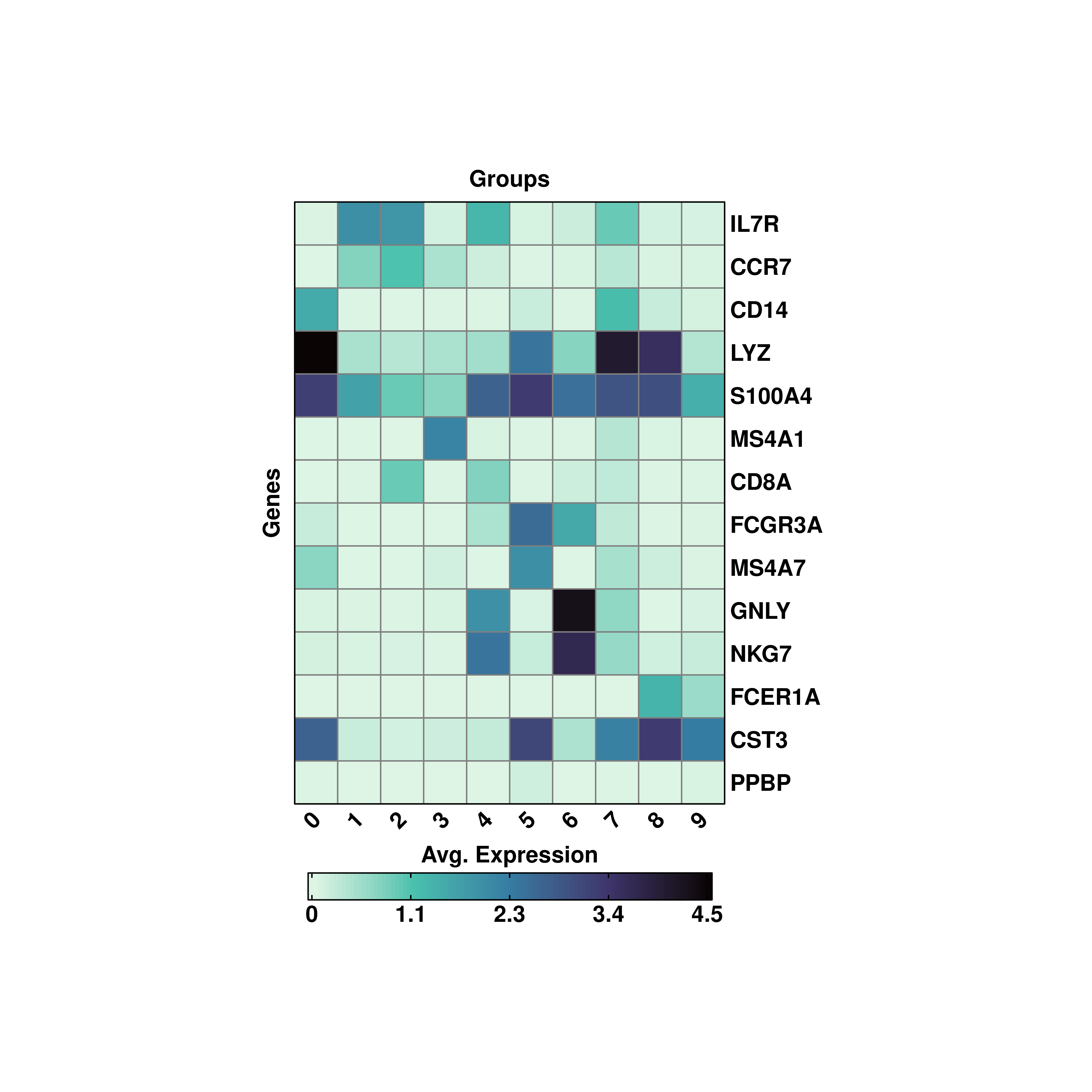
19.4 Modify the rotation of row and column titles
Both rows and column names can be rotated using column_names_rot and row_names_rot parameters, providing the desired angle.
# Rotating the labels.
p <- SCpubr::do_ExpressionHeatmap(sample = sample,
                                  features = genes,
                                  flip = TRUE,
                                  column_names_rot = 0,
                                  viridis_direction = -1)
p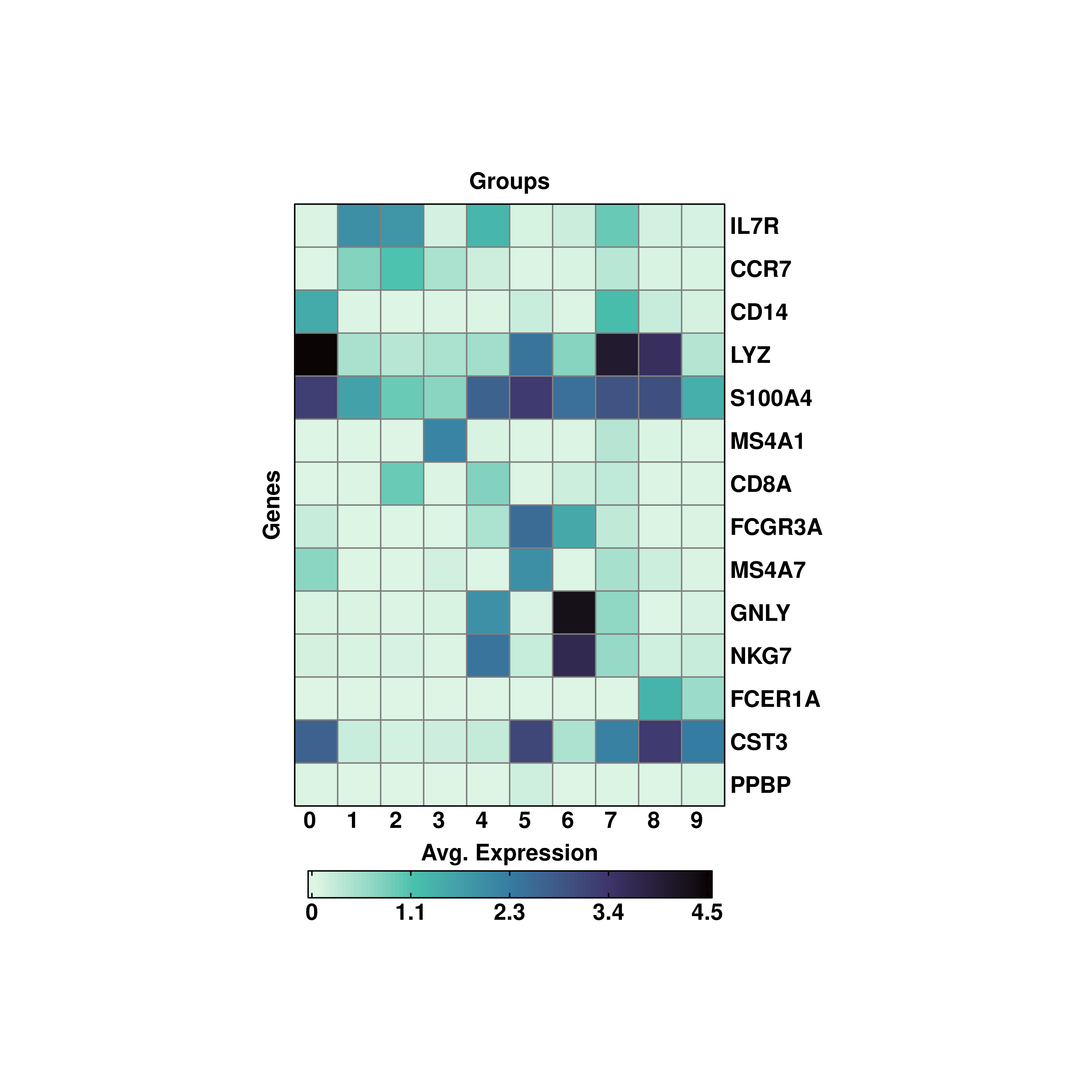
19.5 Changing the cell size in the heatmap.
By design, the aspect ratio of the tiles in the heatmap is fixed so that cells are squares, and not rectangles. However, the user has the possibility to increase/decrease the cell size of each tile by modifying cell_size parameter. This is set to 5 by default.
# Modifying the tile size.
p <- SCpubr::do_ExpressionHeatmap(sample = sample,
                                  features = genes,
                                  flip = TRUE,
                                  cluster_cols = FALSE,
                                  cluster_rows = TRUE,
                                  cell_size = 10,
                                  viridis_direction = -1)
p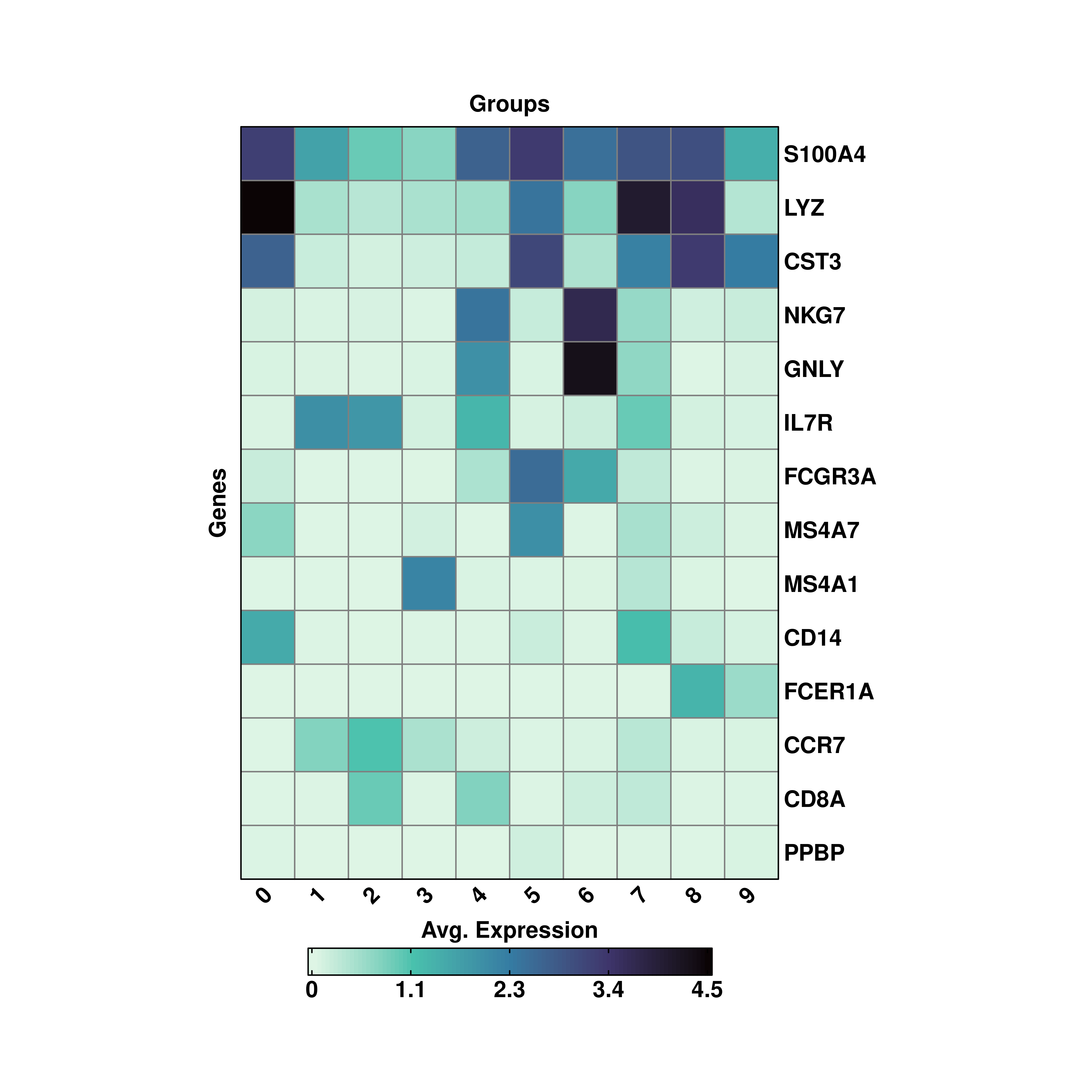
19.6 Symmetrical scales
If one wants a symmetrical scale,
# Symmetrical scale viriis.
p <- SCpubr::do_ExpressionHeatmap(sample = sample,
                                  features = genes,
                                  flip = TRUE,
                                  cluster_cols = FALSE,
                                  cluster_rows = TRUE,
                                  enforce_symmetry = TRUE)
p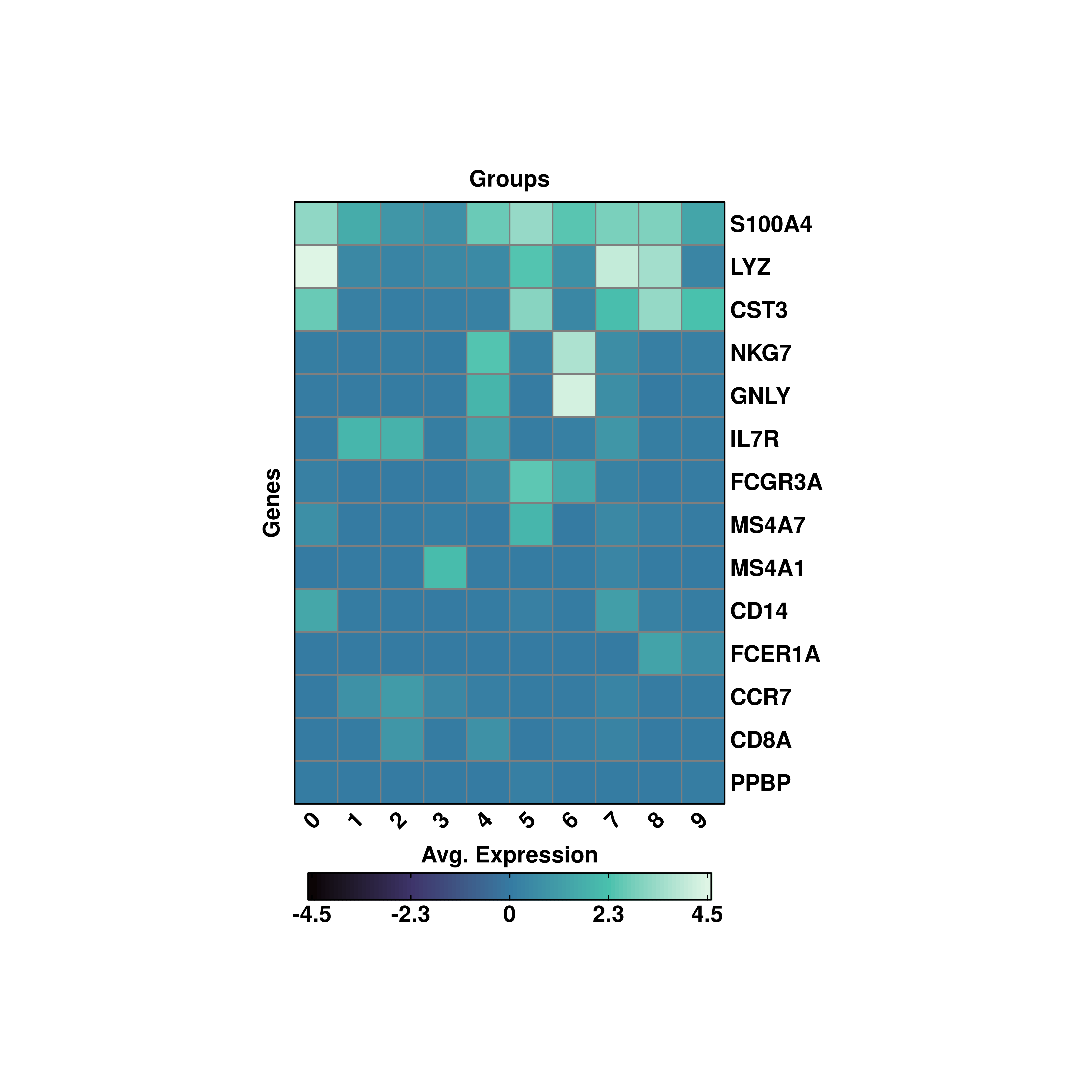
For such cases, it is best to set use_viridis = FALSE.
# Modifying the symmetrical scale non viridis.
p <- SCpubr::do_ExpressionHeatmap(sample = sample,
                                  features = genes,
                                  flip = TRUE,
                                  cluster_cols = FALSE,
                                  cluster_rows = TRUE,
                                  enforce_symmetry = TRUE,
                                  use_viridis = FALSE)
p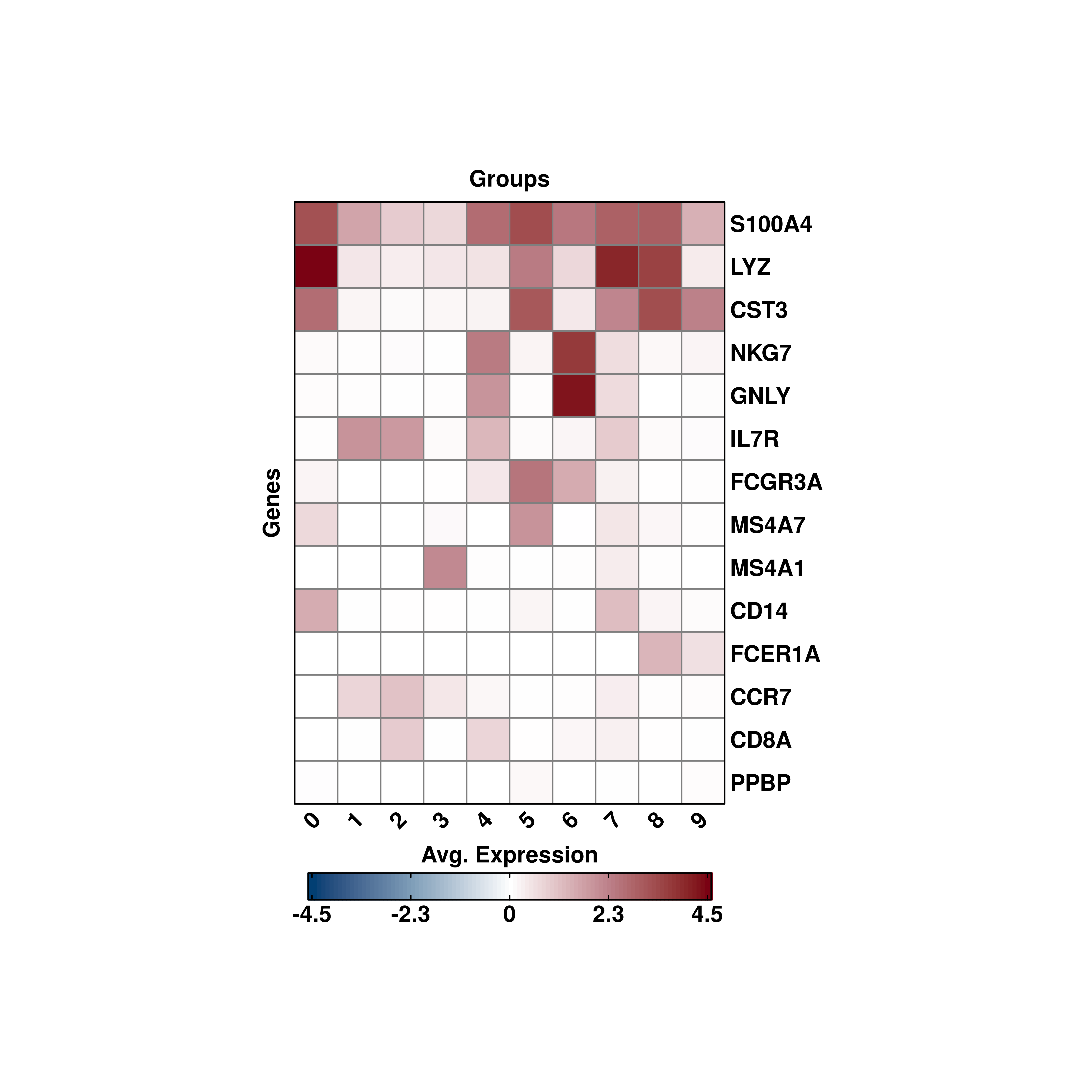
19.7 Subset the color scale.
It might be the case that a single gene set, for a single cluster, drives the color scale entirely. We can treat this as an outlier, so that we can subset the color scale to better represent the values in between. We can achieve that by using min.cutoff and/or max.cutoff.
# Subset the color scale.
p <- SCpubr::do_ExpressionHeatmap(sample = sample,
                                  features = genes,
                                  flip = TRUE,
                                  cluster_cols = FALSE,
                                  cluster_rows = TRUE,
                                  min.cutoff = 0.2,
                                  max.cutoff = 0.7,
                                  viridis_direction = -1)
p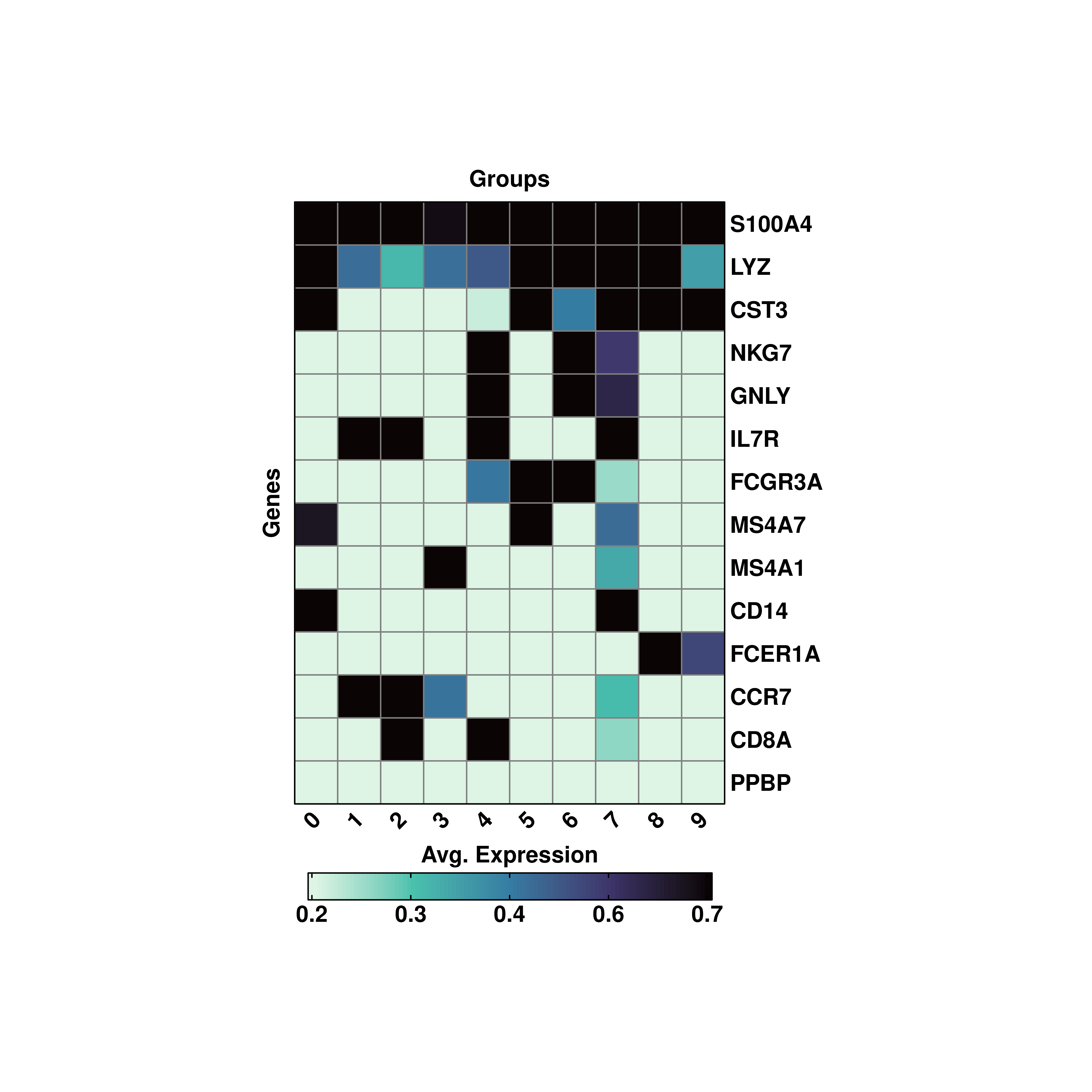
19.8 Use of metadata variables
By design, this function expects to work with expression values, as the overall idea of the plot is to assess similarities/differences between averaged expression levels. However, it might be the case that you might have some metadata values that you would also like to plot in a similar way.
Here is a workaround to make that possible:
# Vector of features stored in the metadata.
my_features <- c("A", "B", "C")

# Retrieve your scores.
scores <- sample@meta.data[, my_features]

# Turn it into a matrix (metadata columns become the features - rows, cells remain as columns).
scores <- t(as.matrix(scores))

# Create an assay object.
scores_assay <- Seurat::CreateAssayObject(counts = scores)

# Add it to your Seurat object.
sample@assays$my_new_assay <- scores_assay

# Plot the features.
p <- SCpubr::do_ExpressionHeatmap(sample = sample,
                                  features = my_features,
                                  assay = "my_new_assay")
p