14 Volcano plots
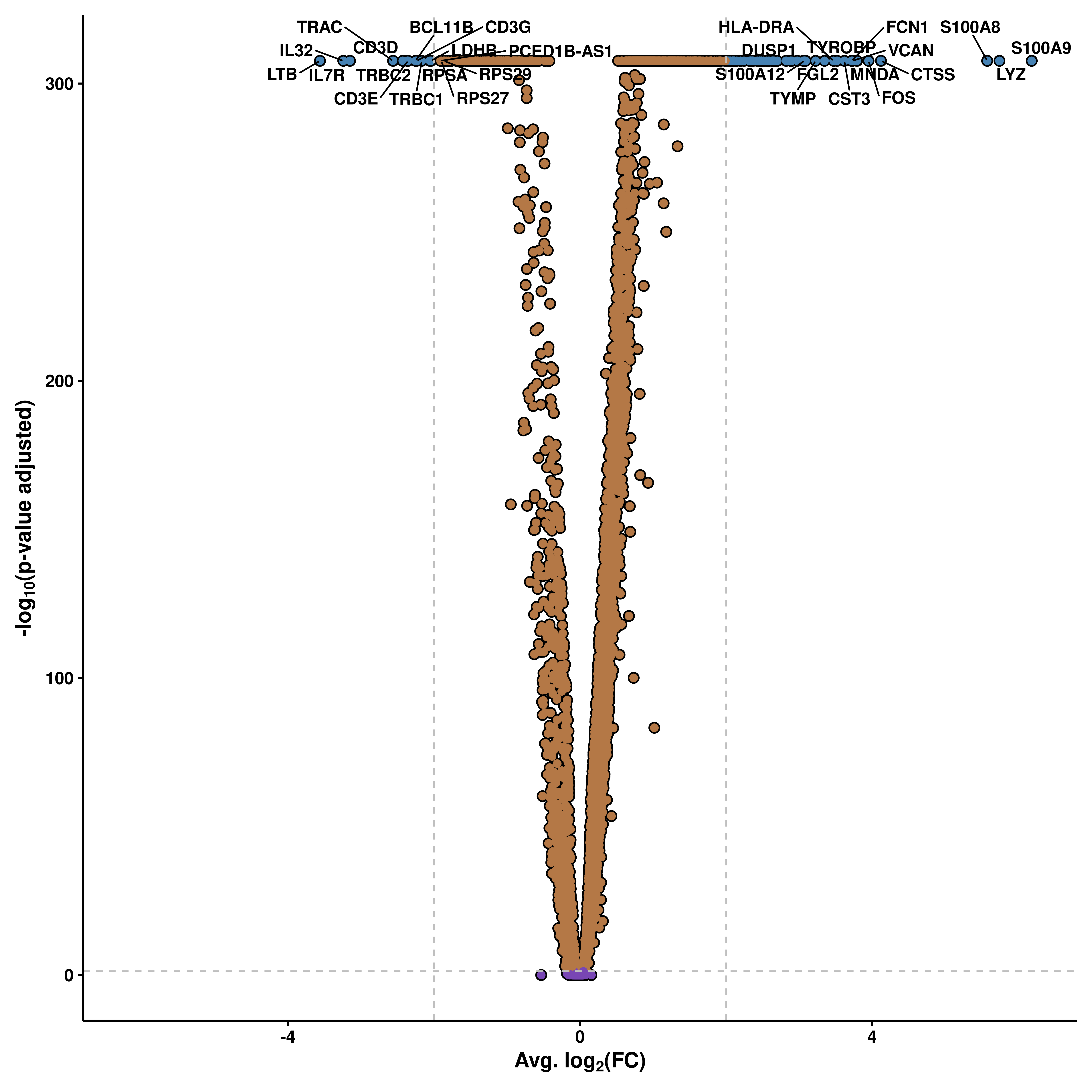
Perhaps one of the most known type of plots for bulk transcriptomics. By computing DE genes across two conditions, the results can be plotted as a volcano plot. This plot features the genes as dots, and places them in a scatter plot where the X axis contains the degree in which a gene is differentially expressed (average log2(FC)), while the Y axis shows the how significant the gene is (-log10(p-value adjusted)).
14.1 Basic usage
To generate such a plot, one can use SCpubr::do_VolcanoPlot(), which needs as input the Seurat object and the result of running Seurat::FindMarkers() choosing two groups.
# Generate a volcano plot.
p <- SCpubr::do_VolcanoPlot(sample = sample,
                            de_genes = de_genes)
p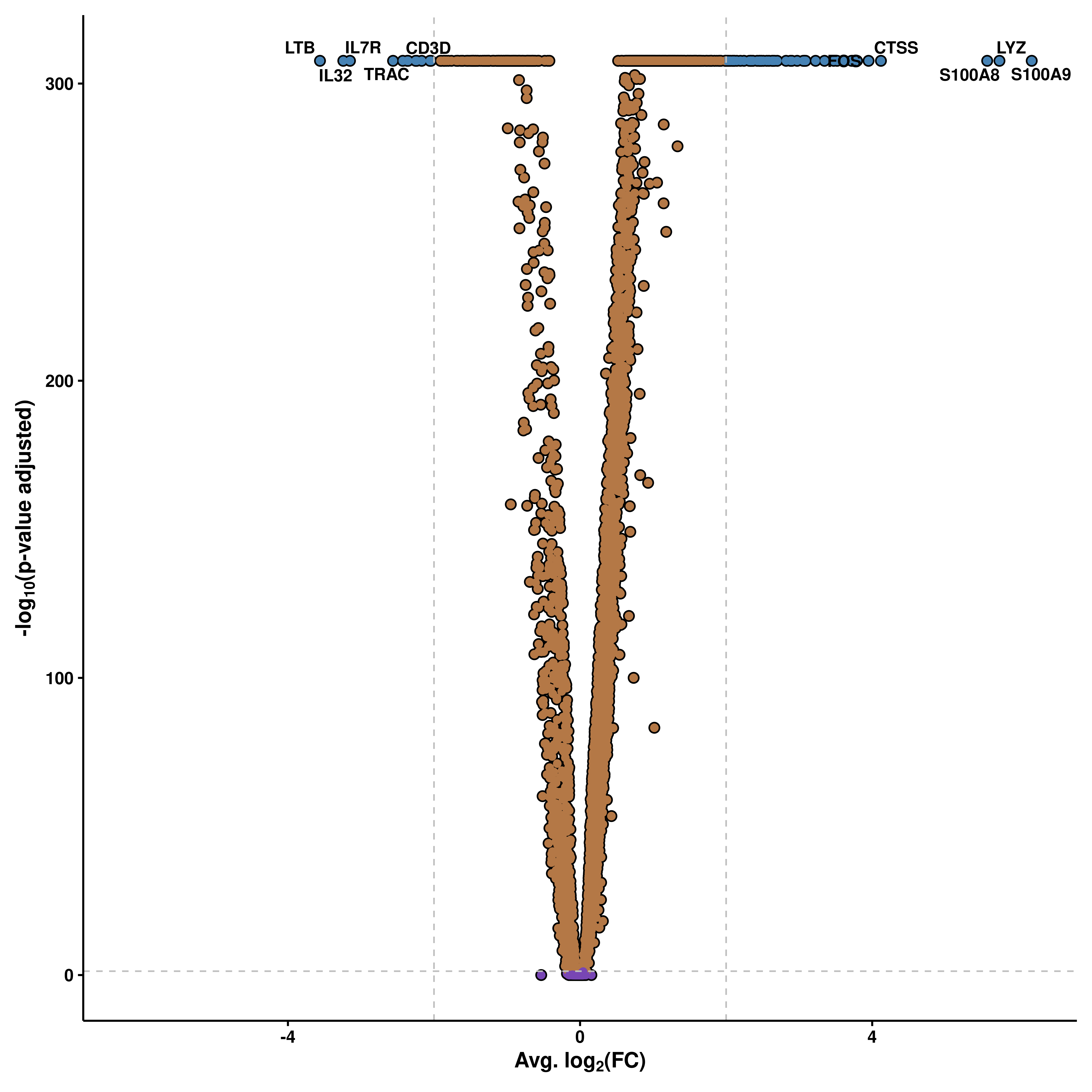
As you can see, there are four major groups of genes: - Genes that surpass our p-value and logFC cutoffs (blue). - Genes that surpass the p-value cutoff but not the logFC cutoff (orange). - Genes that surpass the logFC cutoff but not the p-value cutoff (purple, not shown). - Genes that do not surpass any cutoff (green).
14.2 Modify the cutoffss
The cutofss can be set up by the user using pval_cutoff (without -log10 transforming) and FC_cutoff (avg log2(FC)).
# Modify cutoffs.
p <- SCpubr::do_VolcanoPlot(sample = sample,
                            de_genes = de_genes,
                            pval_cutoff = 1e-50,
                            FC_cutoff = 0.2)
p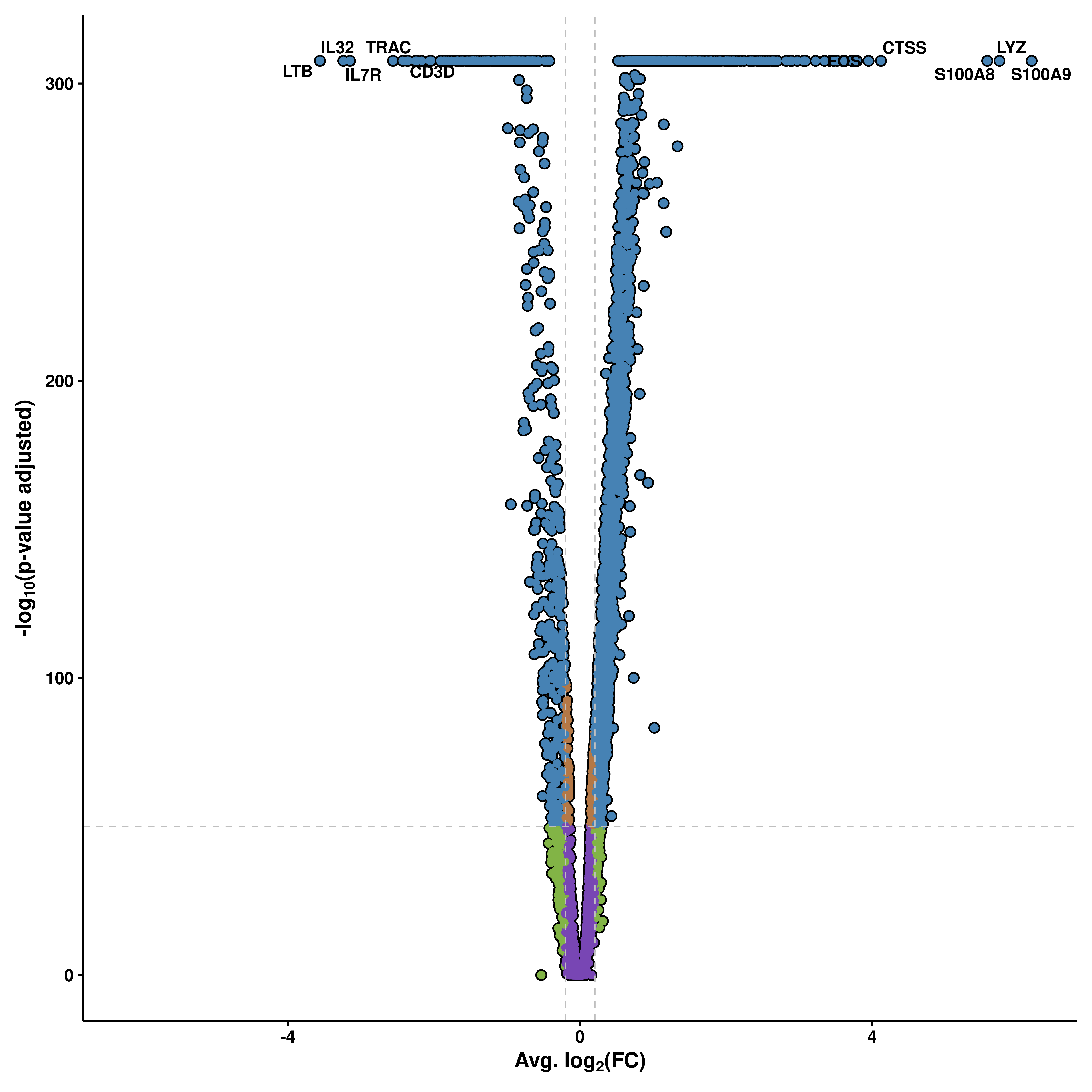
14.3 Modify the gene tags
By default, the top 5 genes on each side, ordered by -log10(p-value adjusted) and average log2(FC) are reported. However, one can increase the number by using
# Modify number of gene tags.
p <- SCpubr::do_VolcanoPlot(sample = sample,
                            de_genes = de_genes,
                            n_genes = 15)
p